Genetic competition in crop breeding trials

Introduction

This vignette describes the complete workflow for considering genetic competition in crop breeding trials using gencomp. More details about the theory underlying gencomp can be found at Stringer, Cullis, and Thompson (2011) and Chaves et al. (2025).

To begin, load gencomp using the code below. Note that gencomp has a strong dependency on asreml, which is a package that is not freely available. Thus, it is vital that asreml is installed. The ggplot2 (Wickham 2016) library will also be loaded for customizing the plots. This is not mandatory.

library(gencomp)
library(ggplot2)

Data description

gencomp has two available datasets. The representative for crop breeding is called potato, obtained from the package agridat Wright (2024). Originally, this dataset was generated by Connolly et al. (1993) to study the inter-plot competition in single-drill plot trials of potatoes in Scotland. They measured the tuber yield of 20 varieties (column gen), which were replicated four times (column rep). Each replication was an independent row of 20 drills. The maturity class of each variety was also registered (column matur), with representatives of the first early (M1), second early (M2) and maincrop (M3) classes. Each drill had five tubers spaced 45 cm apart, with 75 cm between drills. The rows (replications) are not contiguous, which impedes the usage of an autocorrelation structure in the residual part of the model. Thus, in this case, we fitted a genetic-competition model considering the within-row competition.

data(potato)
head(potato)

rep	gen	row	col	yield	matur
R1	V10	4	1	13.2	M3
R1	V06	4	2	9.9	M1
R1	V14	4	3	14.0	M3
R1	V13	4	4	8.6	M3
R1	V07	4	5	13.4	M3
R1	V09	4	6	10.7	M3

Building the competition matrix

The competition matrix (or incidence matrix of competition effects), henceforth depicted as $\mathbf{Z}_c$ is indispensable for the analysis. In the case of crop breeding, $\mathbf{Z}_c$ will be an incidence matrix with ones in the positions corresponding to the genotypes neighboring a given plot in the horizontal or vertical directions, and zero elsewhere Stringer, Cullis, and Thompson (2011). To build the $\mathbf{Z}_c$ , gencomp has the function prepcrop. Here is how to use it employing the example dataset:

comp_mat = prepcrop(
  data = potato,
  gen = "gen",
  row = "row",
  col = "col",
  plt = NULL,
  effs = c("rep", 'matur'),
  trait = "yield",
  direction = "row",
  verbose = TRUE
)

data is the working dataset. gen, row, col, and trait are the column names in the dataset that contain the information of genotypes, row, column, and trait, respectively. The plt argument is optional (defaulting to NULL) and allows users to specify the name of the column containing plot information. This helps ensure that the functions follow the same order as the data collection in the field. If plt is not provided, the function will automatically generate a column to differentiate the plots, ordering the dataset by row and column. The effs argument accepts a string vector with the names of columns representing other effects to be considered in the model fitting step. For instance, the effect of block (rep) and maturity stage (matur). direction defines which direction will be considered (row column) for constructing the competition matrix. Finally, verbose controls whether a progress bar is printed in the console or not.

The prepcrop function generates a list of class comprepcrop. This list has three elements:

A data frame with the inputted data and $\mathbf{Z}_c$ merged:

comp_mat$data[1:5, c(1:5, (ncol(comp_mat$data)-4):ncol(comp_mat$data))]

V02	V03	gen	row	col	yield	matur
0	1	V11	1	1	14.2	M3
0	0	V03	1	2	11.6	M1
0	1	V12	1	3	15.7	M3
1	0	V20	1	4	12.8	M2
0	0	V02	1	5	9.6	M1

A data frame containing the phenotypic records of each focal tree and its neighbors:

head(comp_mat$neigh_check)

gen	row	col	y_focal	y_row
V11	1	1	14.2	11.60
V03	1	2	11.6	14.95
V12	1	3	15.7	12.20
V20	1	4	12.8	12.65
V02	1	5	9.6	13.60
V07	1	6	14.4	10.15

The $\mathbf{Z}_c$ per se:

comp_mat$Z[1:5, 1:5]

V01	V02	V03	V04	V05
0	0	1	0	0
0	0	0	0	0
0	0	1	0	0
0	1	0	0	0
0	0	0	0	0

comprepcrop objects are compatible with the S3 method plot, which can be used to generate a heatmap illustrating the field trial, and box-plots with each candidate’s performance.

plot(comp_mat, category = "heatmap")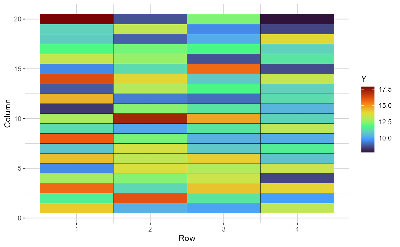

Heatmap representing the grid, in which the cells are filled according to the phenotype value of each plot (blank cells are missing values)


plot(comp_mat, category = "boxplot")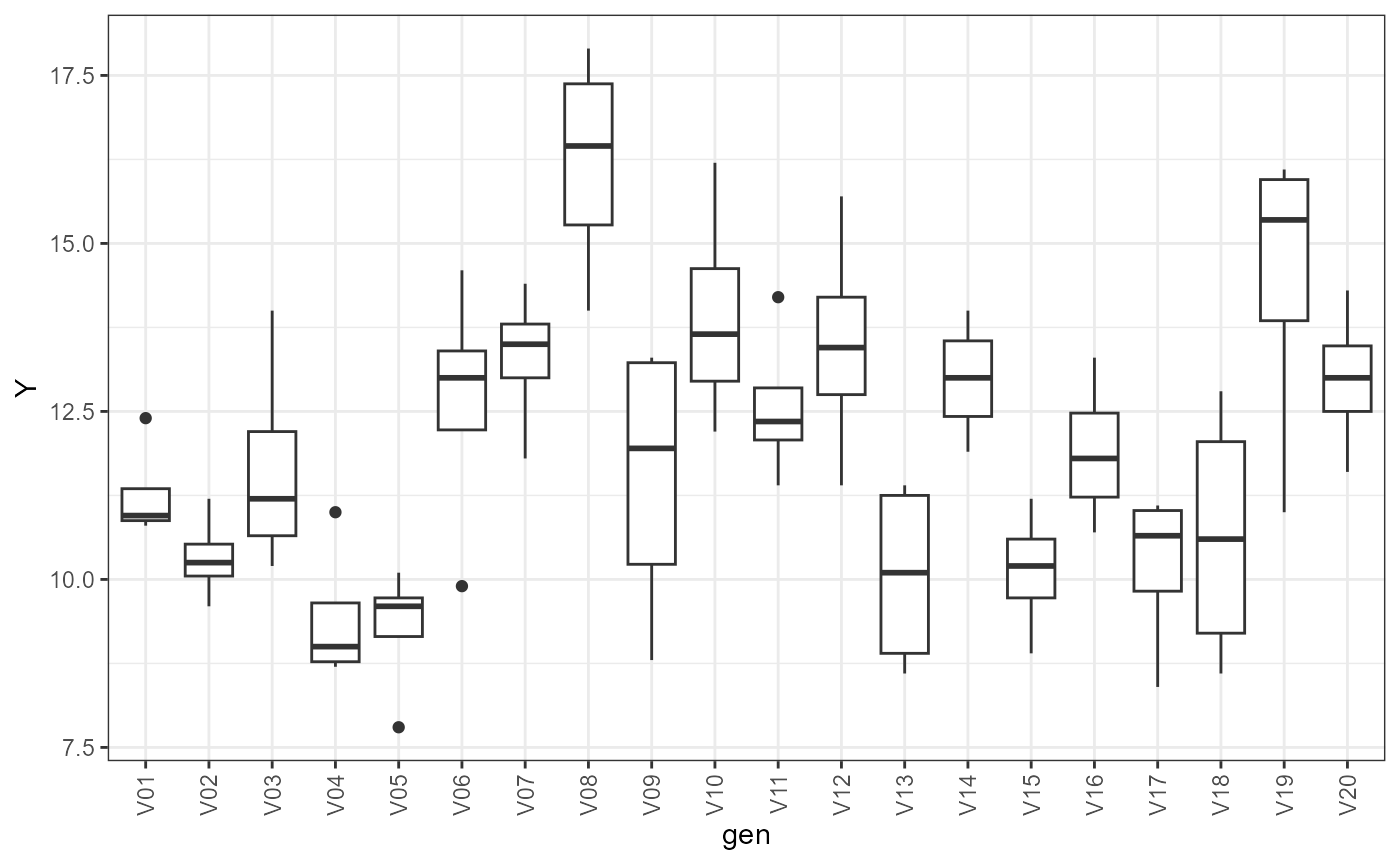

Boxplots depicting the phenotypic performance (y-axis) of each selection candidate (x-axis).

The summary(comprepfor) function returns the number of phenotypic records, number of selection candidates, number of rows and columns, and the direction that is being considered.

summary(comp_mat)
#>   yield gen row col direction
#> 1    80  20   4  20       row

Fitting the model

A general spatial-genetic competition model can be represented by:

$\mathbf{y} = \mathbf{X} \boldsymbol{\beta} + \mathbf{Z}_g \mathbf{g} + \mathbf{Z}_c \mathbf{c} + \mathbf{Z}_p \mathbf{p} + \boldsymbol{\varepsilon}$

where $\mathbf{y}$ is the vector of phenotypic records, $\boldsymbol{\beta}$ is the vector of fixed effects, $\mathbf{g}$ is the vector of direct genetic effects (DGE), $\mathbf{c}$ is the vector of indirect genetic effects (IGE), $\mathbf{p}$ is the vector of other random effects, and $\boldsymbol{\varepsilon}$ is the vector of spatially correlated errors. $\mathbf{X}$ is the incidence matrix of the fixed effects, $\mathbf{Z}_g$ is the DGE incidence matrix, $\mathbf{Z}_c$ is the IGE incidence matrix (built using prepfor), and $\mathbf{Z}_p$ is the design matrix of other random effects. The dimensions of $\mathbf{Z}_c$ are the same as $\mathbf{Z}_g$ . The spatially correlated errors are distributed as $\boldsymbol{\varepsilon} \sim \mathcal{N}\{\mathbf{0}, \sigma^2_\varepsilon[\mathbf{AR1}(\rho_C) \otimes \mathbf{AR1}(\rho_R)]\}$ , where $\sigma^2_\varepsilon$ is the spatially correlated residual variance, $\mathbf{AR1}(\rho_C)$ and $\mathbf{AR1}(\rho_R)$ are the first-order autoregressive correlation matrices in the column and row directions, and $\otimes$ is the Kronecker product. Note that spatial modelling is not possible in the example dataset, so $\boldsymbol{\varepsilon} \mathcal{N} \left( \mathbf{0}, \sigma^2_\varepsilon \mathbf{I} \right)$ , i.e., a genetic competition model (without the spatial component) is being fitted. If cor = TRUE (default, see below), the function will fit a model in which $\mathbf{g}$ and $\mathbf{c}$ are correlated outcomes of the genotypic effects decomposition. They both follow a Gaussian distribution, with mean centred in zero, and covariance given by:

$\mathbf{\Sigma_g} = \begin{bmatrix}\sigma_{\text{g}}^2 & \sigma_{\text{gc}}\\\sigma_{\text{gc}} & \sigma_{\text{c}}^2\\\end{bmatrix}\otimes {{\mathbf I_V}}$

where $\sigma_{\text{g}}^2$ is the DGE variance, $\sigma_{\text{c}}^2$ is the IGE variance, and $\sigma_{\text{gc}}$ is the covariance between DGE and IGE. An alternative parametrization considers that $\mathbf{g}$ and $\mathbf{c}$ are independent. If this is not true for the trait and/or population under investigation, assuming independence will add bias to the results.

The function that fits the genetic-competition linear mixed model uses the average information algorithm implemented in the asreml package (The VSNi Team 2023). Check the function’s structure using the example dataset:

model = asr(
  prep.out = comp_mat,
  fixed = yield ~ rep + matur,
  random = ~ 1,
  lrtest = TRUE,
  spatial = FALSE,
  cor = TRUE
)

prep.out is a comprepcrop object. fixed is a formula, declared just like is usually done for regular asreml models. random is also a formula, but this argument should just be altered if other random effects than the genotypic effects should be considered in the model. This is because all pre-programmed models already consider DGE and IGE, as previously described. lrtest defines if hypothesis tests using likelihood ratio tests should be done. spatial determines if a regular genetic competition model (spatial = FALSE) or a spatial-genetic competition model (spatial = TRUE) should be fitted. Finally, cor dictates if the function will fit a model considering the covariance between DGE and IGE (cor = TRUE) or not (cor = FALSE). asr can receive other arguments passed on to the asreml function (see ?asreml for more information). The output of the asr function is an object of classes asreml and compmod. Since it holds the asreml class, it is suitable for using with S3 methods like plot, summary, predict, update, resid and others (see help("asreml.object")).

Extracting the results

The function to obtain the main results from the compmod object is called resp, and its structure is exemplified below using the example dataset:

res = resp(
  prep.out = comp_mat,
  model = model,
  weight.tgv = FALSE,
  sd.class = 1
)

model is the compmod object obtained from the asr function. weight.tgv receives a logical value, and determines if the reliability should be used as weight to compute the total genotypic value (TGV) or not. sd.class is a weight to multiply the standard deviation of competition effects when determining the competition classes (defaults to 1). The resp function returns an object (list) of classes comresp and comprepcrop. This object is compatible with the S3 methods plot, print and summary. A detailed description of the results within the list generated by res is provided below.

Variance components

The data frame with the variance components will yield different results depending on the model. cor(IGE_DGE), which represents the correlation between DGE and IGE; DGE and IGE will always be present in variance component obtained from compmod objects. The residuals will have different forms depending if spatial is TRUE or FALSE in the asr function.

res$varcomp

	component	std.error	z.ratio	bound	%ch
cor(IGE_DGE)	-0.8012	0.1791	-4.4744	U	0.3
DGE	2.9292	1.1294	2.5936	P	0.3
IGE	0.4616	0.2108	2.1898	P	0.0
R	0.9875	0.2266	4.3579	P	0.0

Likelihood ratio tests

Available only if lrt = TRUE in the asr function.

res$lrt

effect	LR-statistic	Pr(Chisq)
DGE	41.62410	0.00e+00
IGE	14.98519	5.42e-05

Heritabilities

Available if cor = TRUE in the function asr. Contain the DGE heritability and total heritability Bijma, Muir, and Van Arendonk (2007). The first is the portion of the total variance that refers to the DGE. The latter is a ratio between the sum of the total heritable components against the phenotypic variance, and it is an adjusted estimate of the heritability that considers the competition effects and the covariance between DGE and IGE. The expressions for these heritabilities are given below:

$H^2_g = \frac{\hat{\sigma}^2_g}{\hat{\sigma}^2_y}$ $H^2_t = \frac{\hat{\sigma}^2_g + 2\times \hat{\phi} \times \hat{\sigma}_{gc} + \hat{\phi}^2 \times \hat{\sigma}^2_c}{\hat{\sigma}^2_y}$ with $\sigma^2_y$ being the total phenotypic variance, and $\hat{\phi}$ the mean competition intensity factor, which, in the case of crop breeding, we assume to be 1 since there is no distance-based weighting.

res$heritability

	Heritability
H2direct	0.669
H2total	0.349

BLUPs

When genetic competition effects are statistically significant, the most appropriate selection unit is the TGV, given by:

${TGV}_v = \hat{g}_v + \hat{\phi} \times \hat{c}_v$ where $\hat{g}_v$ and $\hat{c}_v$ are the DGE and IGE of the $v^{th}$ candidate, respectively. If weight.tgv = TRUE in the resp function, the weighted TGV is computed as follows:

${wTGV}_v = \hat{g}_v \times r_{g_v}^2 + \hat{\phi} \times \hat{c}_v \times r_{c_v}^2$ with $r_{g_v}^2$ and $r_{c_v}^2$ being the reliabilities of DGE and IGE, respectively.

The comresp object has a data frame containing the DGE and IGE, their standard errors, the competition class of each genotype and the TGV. If other random effects were declared in the model, there will be a further data frame with their BLUPs.

head(res$blups$main)

gen	DGE	se.DGE	rel.DGE	IGE	se.IGE	rel.IGE	class	TGV
V08	3.903	0.624	0.867	-1.207	0.329	0.765	Aggressive	2.696
V19	2.186	0.657	0.852	-0.757	0.329	0.766	Aggressive	1.429
V20	0.832	0.850	0.753	-0.019	0.343	0.745	Homeostatic	0.813
V12	0.834	0.639	0.861	-0.109	0.337	0.755	Homeostatic	0.726
V10	1.296	0.622	0.868	-0.631	0.336	0.756	Aggressive	0.665
V06	0.581	0.768	0.799	-0.057	0.345	0.742	Homeostatic	0.524

From this data frame, several information can be extracted. Check out below.

Competition classes

The higher the IGE, the more aggressive is the genotype. Here, we use a modified version of the classification proposed by Ferreira et al. (2023) to define competition classes:

$\text{Classes} = \begin{cases} \bar{c} - (\tau) sd(c) < \hat{c}_v < \bar{c} + (\tau) sd(c) \rightarrow \text{Homoeostatic} \\ \hat{c}_v > \bar{c} + (\tau) sd(c) \rightarrow \text{Sensitive} \\ \hat{c}_v < \bar{c} - (\tau) sd(c) \rightarrow \text{Aggresive} \end{cases}$ with $\bar{c}$ being the mean IGE in the population, $\hat{c}_v$ the IGE of the $v^{th}$ genotype, $sd(c)$ the IGE’s standard deviation, and $\tau$ a weight defining the thresholds to declare if a genotype is aggressive, homoeostatic or sensitive.

This classification is illustrated using a density plot, a scatter plot and a heat map representing the field grid. These plots aid in the investigation of the relationship between DGE and IGE, how this dynamics are related to classification, and how aggressive, homoeostatic and sensitive are distributed in the field.

plot(res, category = "class")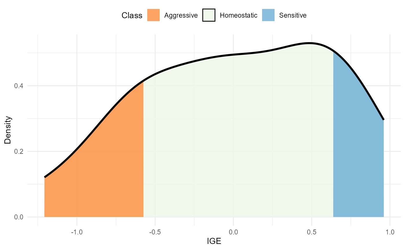

Density of IGE values. The area within the distribution is filled according to the competition class

plot(res, category = "DGEvIGE")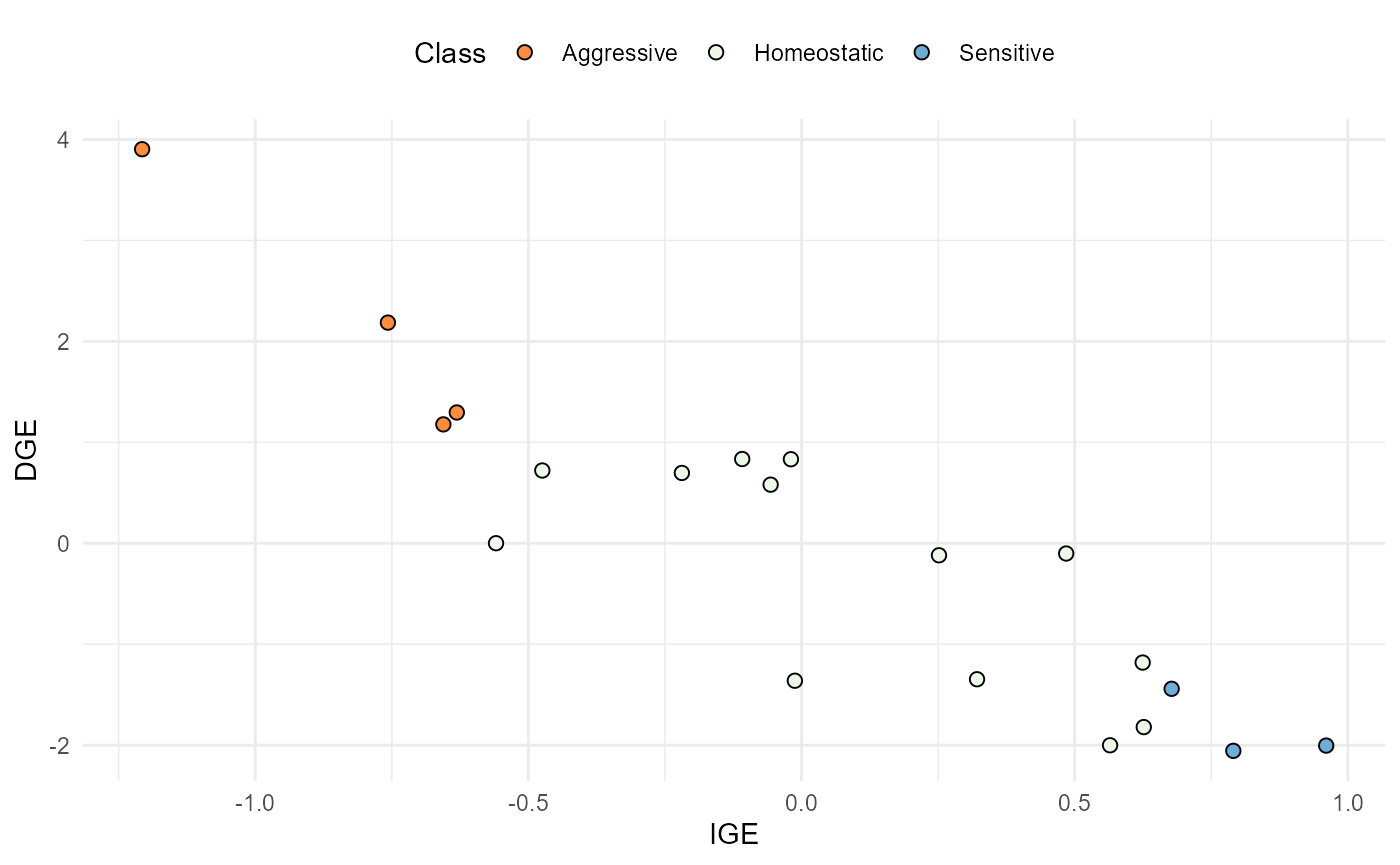

Relationship between IGE (x-axis) and DGE (y-axis). The dots are coloured according to the competition class.

plot(res, category = "grid.class")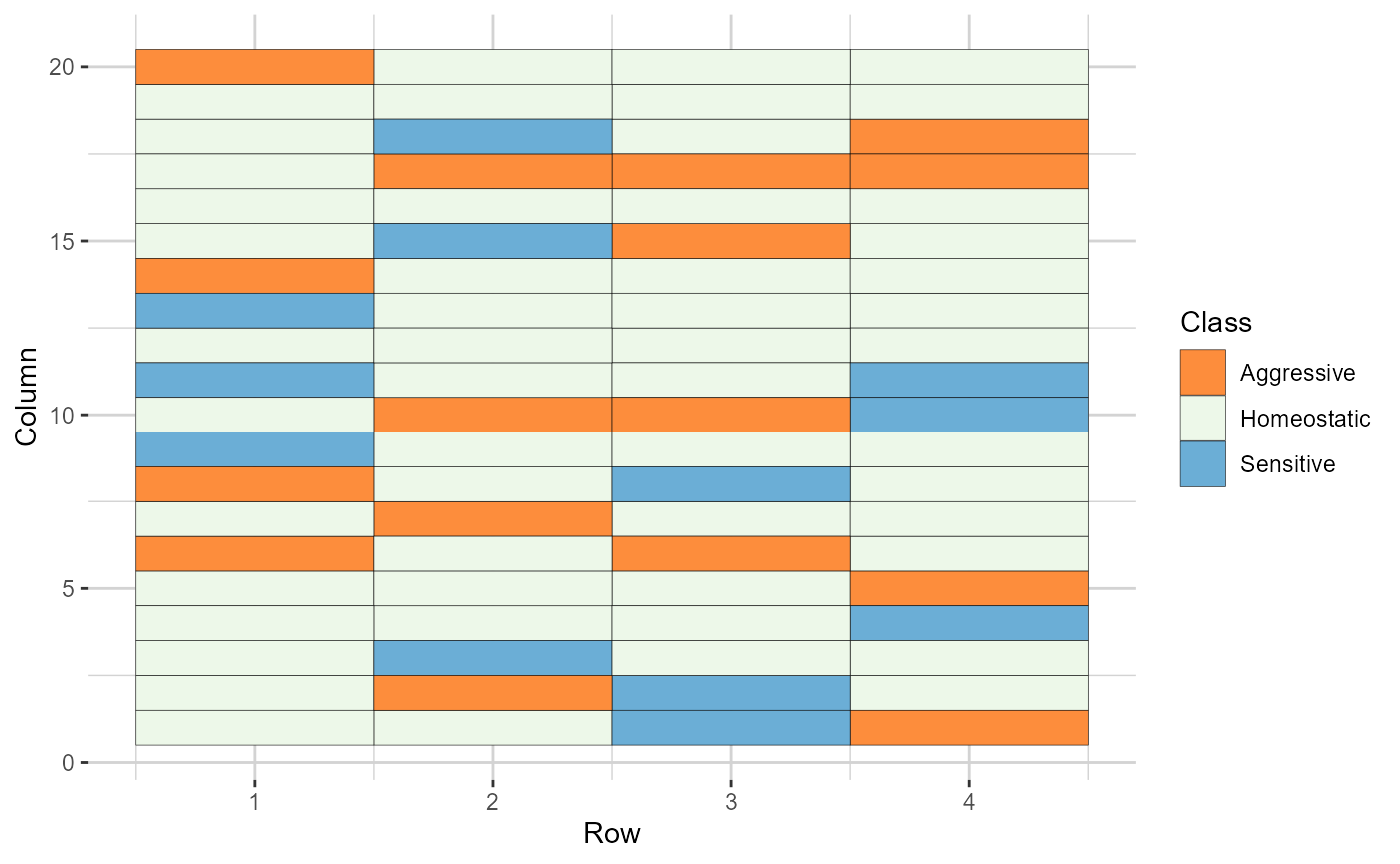

Heatmap representations of the field trial, with cells filled according to the competition class of each genotype

Ranking

Three possible rankings are possible: based on the DGE, the IGE, or the TGV. Note that DGE and IGE have different reliabilities, with DGE’s being usually higher. It is advisable to take this into consideration when making decisions.

plot(res, category = "DGE.IGE")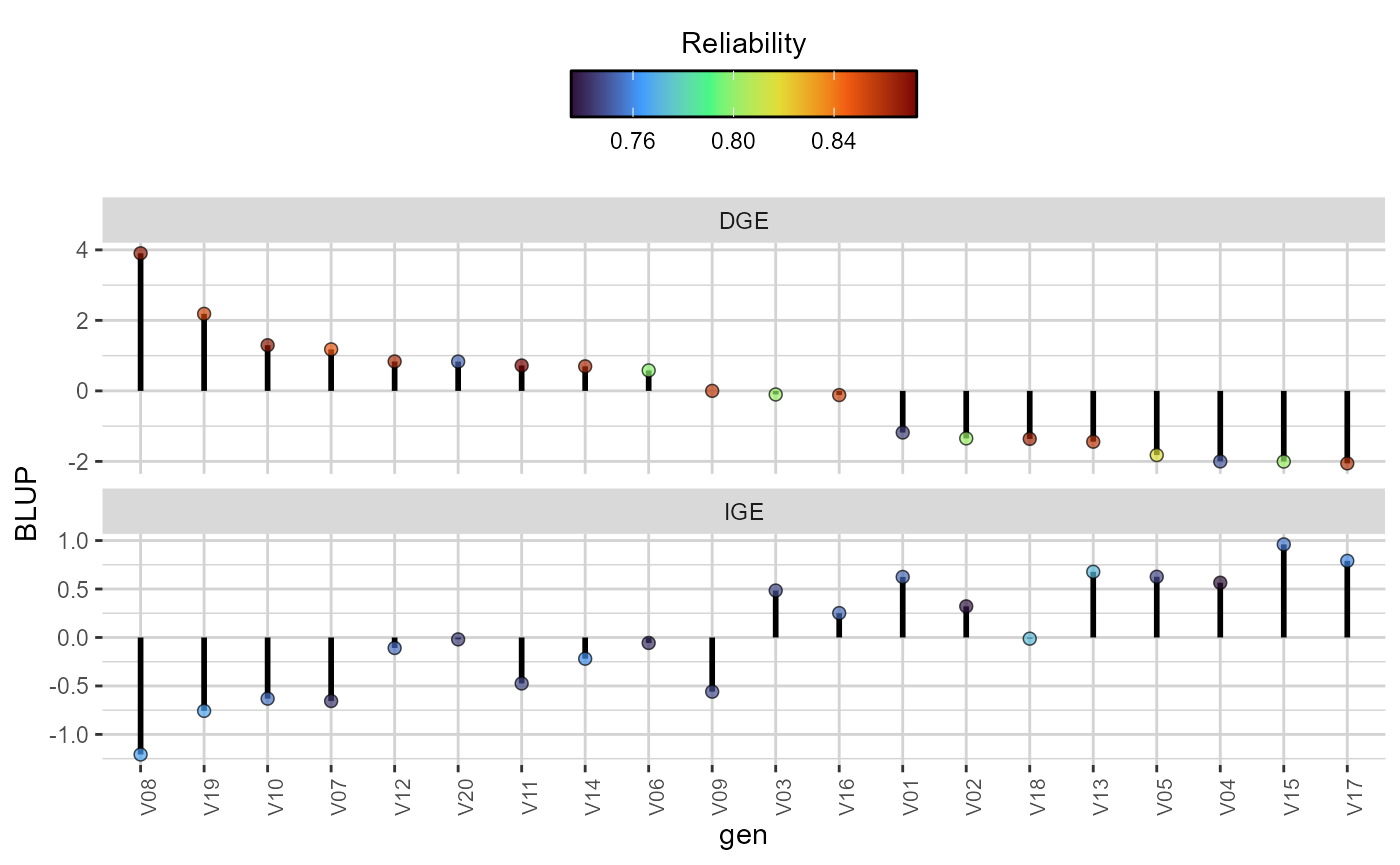

Direct (DGE) and indirect (IGE) genotypic effects ( extit{y}-axis) of each candidate. The plots are in descending order according to the DGE. The colour of the dots reflects the reliability of both the DGE and IGE for each genotype

plot(res, category = "TGV")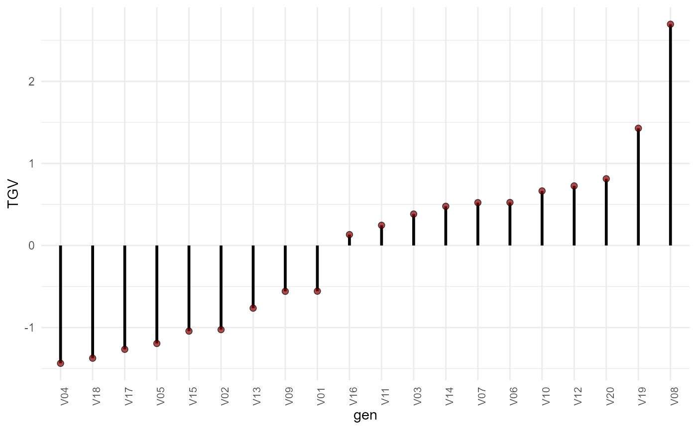

Total genotypic value (TGV) (y-axis) of each candidate (x-axis), in increasing order

The distribution of high-performance and/or competitive candidates is also illustrated.

plot(res, category = "grid.dge")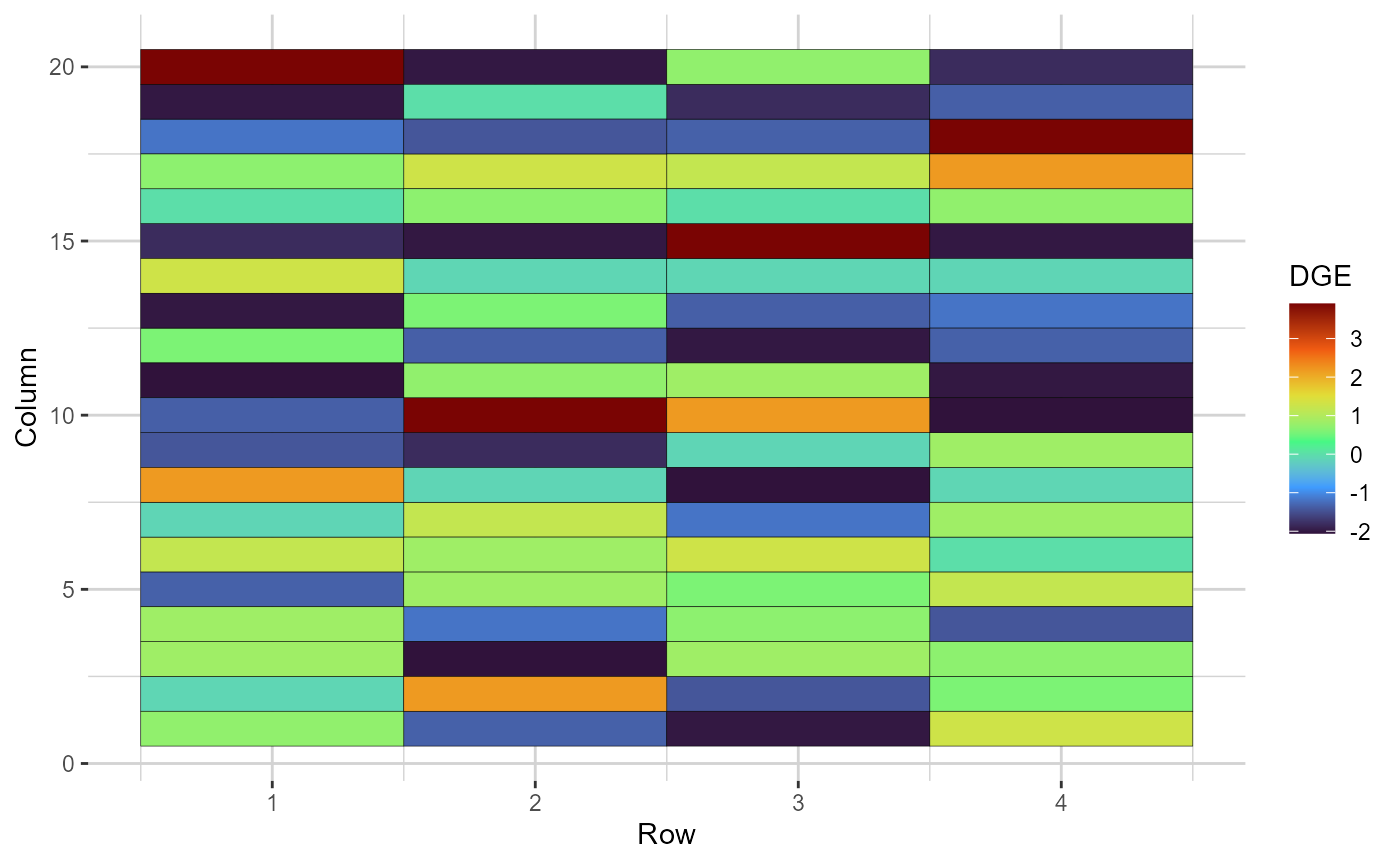

Heatmap representations of the field trial, with cells filled according to the direct genotypic effect (DGE) of each genotype

plot(res, category = "grid.ige")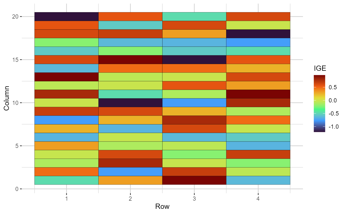

Heatmap representations of the field trial, with cells filled according to the indirect genotypic effect (IGE) of each genotype

Error distribution

The last plot available for objects of class compresp is a heatmap coloured according to the residual value of each plot. This is useful to observe possible trends in the field.

plot(res, category = "grid.res")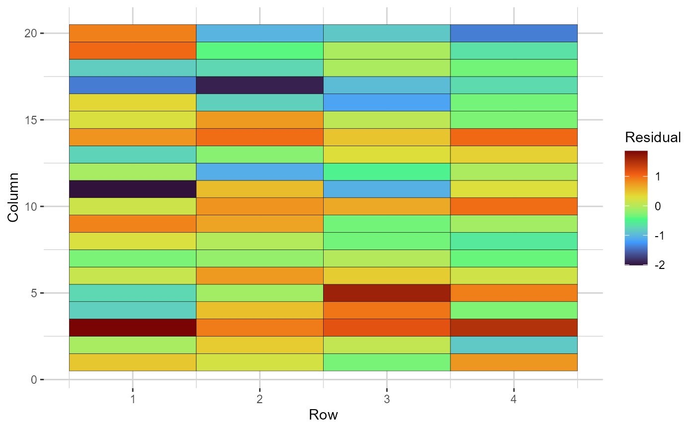

Heatmap representations of the field trial, with cells filled according to the residual value of each plot. Blank cells are missing values

References

Bijma, Piter, William M. Muir, and Johan A. M. Van Arendonk. 2007. “Multilevel Selection 1: Quantitative Genetics of Inheritance and Response to Selection.” Genetics 175 (1): 277–88. https://doi.org/10.1534/genetics.106.062711.

Chaves, Saulo F. S., Filipe M. Ferreira, Getulio C. Ferreira, Salvador A. Gezan, and Kaio Olimpio G. Dias. 2025. “Incorporating Spatial and Genetic Competition into Breeding Pipelines with the R Package Gencomp.” Heredity, January, 1–13. https://doi.org/10.1038/s41437-024-00743-9.

Connolly, T, I D Currie, J E Bradshaw, and J W McNicol. 1993. “Inter‐plot Competition in Yield Trials of Potatoes (Solanum Tuberosum L.) with Single‐drill Plots.” Annals of Applied Biology 123 (2): 367–77. https://doi.org/10.1111/j.1744-7348.1993.tb04099.x.

Ferreira, Filipe M., Saulo F. S. Chaves, Leonardo L. Bhering, Rodrigo S. Alves, Elizabete K. Takahashi, João E. Sousa, Marcos D. V. Resende, et al. 2023. “A Novel Strategy to Predict Clonal Composites by Jointly Modeling Spatial Variation and Genetic Competition.” Forest Ecology and Management 548: 121393. https://doi.org/10.1016/j.foreco.2023.121393.

Stringer, Joanne K., Brian R. Cullis, and Robin Thompson. 2011. “Joint Modeling of Spatial Variability and Within-Row Interplot Competition to Increase the Efficiency of Plant Improvement.” Journal of Agricultural, Biological, and Environmental Statistics 16 (2): 269–81. https://doi.org/10.1007/s13253-010-0051-5.

The VSNi Team. 2023. Asreml: Fits Linear Mixed Models Using REML. www.vsni.co.uk.

Wickham, Hadley. 2016. Ggplot2: Elegant Graphics for Data Analysis. Springer-Verlag New York. https://ggplot2.tidyverse.org.

Wright, Kevin. 2024. Agridat: Agricultural Datasets. https://CRAN.R-project.org/package=agridat.

Saulo F. S. Chaves

2025-01-21