Genetic competition in tree breeding trials: repeated measures

Introduction

This vignette describes the workflow for considering genetic competition in a repeated measures context, in tree breeding trials, using gencomp. More details about the theory underlying gencomp can be found at Filipe Manoel Ferreira et al. (2024) and Chaves et al. (2025).

To begin, load gencomp using the code below. Note that gencomp has a strong dependency on asreml, which is a package that is not freely available. Thus, it is vital that asreml is installed. The ggplot2 (Wickham 2016) library will also be loaded for customizing the plots. This is not mandatory.

library(gencomp)
library(ggplot2)

Data description

gencomp has two available datasets. The representative for tree breeding is called euca, whose phenotypes were simulated using parameters from a real data of an intermediate-stage clonal eucalyptus trial. It has the mean annual increment values (m³ ha^-1 year^-1, column MAI) of a total of 100 clones (“C001” to “C100” in clone column) laid out in a randomized complete block design with 13 replicates (“B01” to “B13” in block column). The experimental unit is the same as the observation unit, i.e., there is a single plant per plot. The plants are spaced by 2 and 3 meters in the row and column directions, respectively; and the position of each tree in the field is found in columns row and col. Phenotypes of two ages are available (“3y” and “6y” in age column). This trial was not organized into contiguous blocks: the first six blocks were situated in one area, while the other seven were in another. The dataset includes a column labelled area, distinguishing between these areas. We will use a single age to illustrate gencomp’s pipeline:

data(euca)
head(euca)

age	area	block	clone	tree	dist_row	dist_col	row	col	MAI
3y	A1	B02	C015	104	2	3	40	4	NA
3y	A1	B02	C003	105	2	3	40	5	6.02
3y	A1	B02	C048	106	2	3	40	6	32.13
3y	A1	B02	C034	107	2	3	40	7	27.46
3y	A1	B02	C008	108	2	3	40	8	28.64
3y	A1	B02	C028	109	2	3	40	9	56.42

Building the competition matrix

The competition matrix (or incidence matrix of competition effects), henceforth depicted as $\mathbf{Z}_c$ is indispensable for the analysis. In the case of tree breeding, due to the large area occupied by a single tree and large spacing between trees, the standard procedure is to compute the directional competition intensity factors for each direction by filling the positions corresponding to the candidates neighbouring a focal tree in the respective row of $\mathbf{Z}_c$ . Currently, gencomp has three options for computing the directional competition intensity factors:

Muir (2005) (MU) $\rightarrow$ The competition intensity factors are the inverse of the distance between the focal individual and its neighbors in the diagonal, row and column directions:

$\begin{cases} f_d = \frac{1}{\sqrt{\mathcal{D}^2_r + \mathcal{D}^2_c}} \\ f_r = \frac{1}{\mathcal{D}_r} \\ f_c = \frac{1}{\mathcal{D}_c} \end{cases}$

where $f_r$ , $f_c$ and $f_d$ are the directional competition intensity factors for a given plot (i.e., a given row of $\mathbf{Z}_c$ ) in the row, column and diagonal directions, respectively; $\mathcal{D}_r$ and $\mathcal{D}_c$ are the distance between the focal individual and its neighbors in the row and column directions, respectively.

Cappa and Cantet (2008) (CC) $\rightarrow$ the distance and the number of neighbours in each direction are considered. This method assumes that the distance between the focal individual and its neighbours in the row is the same as the distance between the focal individual and its neighbours in the column:

$\begin{cases} f_d = \frac{1}{\sqrt{2 \left(n_c + n_r\right) + n_d}} \\ f_r = \sqrt{\frac{2}{2 \left(n_c + n_r\right) + n_d}} \\ f_c = \sqrt{\frac{2}{2 \left(n_c + n_r\right) + n_d}} \end{cases}$

where $n_r$ , $n_c$ and $n_d$ are the number of neighbors in the row, column and diagonal directions, respectively

Costa e Silva and Kerr (2013) (SK) $\rightarrow$ considers the number of neighbors, the distance between the focal individual and its neighbors and the difference between distances in the row and column directions:

$\begin{cases} f_d = \frac{p}{\sqrt{\left(n_r p^4 \right) + \left(n_r p^2 \right) + \left(n_c p^2 \right) + \left(n_d p^2 \right) + n_c }} \\ f_r = f_d \sqrt{1 + p^2} \\ f_c = \frac{f_d \sqrt{1 + p^2}}{p} \end{cases}$

where $p = {\mathcal{D}_c}/{\mathcal{D}_r}$ .

Once the direction competition intensity factors are estimated, the mean competition intensity factor ( $\phi$ , or CIF, in the function’s output) is obtained as follows:

$\hat{\phi} = \overline{n_r} \overline{f}_r + \overline{n}_c \overline{f}_c + \overline{n}_d \overline{f}_d$

In the multi-age model, $\mathbf{Z}_c = (\mathbf{Z}_{c_1}, \mathbf{Z}_{c_2}, \dots, \mathbf{Z}_{c_M})$ , i.e., a unique competition matrix must be built for each age level $\left(m = 1, 2, \dots, M\right)$ . To build the $\mathbf{Z}_c$ , gencomp has the function prepfor. Here is how to use it employing the example dataset:

comp_mat = prepfor(
  data = euca,
  gen = 'clone',
  area = 'area',
  plt = 'tree',
  age = 'age',
  row = 'row',
  col = 'col',
  dist.col = 3,
  dist.row = 2,
  trait = 'MAI',
  method = 'SK',
  n.dec = 3,
  verbose = TRUE,
  effs = c("block")
)

data is the working dataset. gen, row, col, and trait are the column names in the dataset that contain the information of genotypes, row, column, and trait, respectively. dist_row and dist_col are the distances between rows and columns, respectively. method refers to the method to be used to compute the competition intensity: it should be "MU", "CC" or "SK" (as detailed above). area and age are NULL by default, but if you have non-contiguous blocks (as we have in our example) and multi-age (repeated measures) data, you can add the name of the columns that contain this information in the data frame. n.dec is the number of decimal digits to show in $\mathbf{Z}_c$ . The plt argument is optional (defaulting to NULL) and allows users to specify the name of the column containing plot information. This helps ensure that the functions follow the same order as the data collection in the field. If plt is not provided, the function will automatically generate a column to differentiate the plots, ordering the dataset by row and column. The effs argument accepts a string vector with the names of columns representing other effects to be considered in the model fitting step. For instance, the effect of block (block). Note that the effect due to age (column age) will be automatically converted to factor. Finally, verbose controls whether a progress bar is printed in the console or not.

The prepfor function generates a list of class comprepfor. This list has the following elements:

A data frame with the inputted data and $\mathbf{Z}_c$ merged:

comp_mat$data[c(1:5, (nrow(comp_mat$data) - 5):nrow(comp_mat$data)),
              c(1:5, (ncol(comp_mat$data)-4):ncol(comp_mat$data))]

C005	dist_row	dist_col	row	col	MAI
0.48	2	3	29	4	24.22
0.40	2	3	29	5	28.05
0.32	2	3	29	6	2.11
0.00	2	3	29	7	24.31
0.00	2	3	29	8	58.35
0.00	2	3	14	42	5.99
0.00	2	3	14	43	3.16
0.00	2	3	14	44	10.85
0.00	2	3	14	45	37.41
0.00	2	3	14	46	NA
0.00	2	3	14	47	59.87

$M$ lists, with each lists containing the following information particularized by age (taking the Age_3y as example):

2.1. A data frame containing the phenotypic records of each focal tree and its neighbors:

head(comp_mat$Age_3y$neigh_check) 
#>    gen row col   y_focal    y_row n_row     y_col n_col    y_diag n_diag
#> 1 C070  29   4 24.221412 28.05104     1       NaN     0  6.466753      1
#> 2 C071  29   5 28.051038 13.16738     2  6.466753     1 19.680433      1
#> 3 C090  29   6  2.113346 26.18276     2 19.680433     1 18.131841      2
#> 4 C096  29   7 24.314490 30.23192     2 29.796930     1 27.012877      2
#> 5 C083  29   8 58.350503 14.37096     2 34.345321     1 29.796930      1
#> 6 C060  29   9  4.427432 39.01547     2       NaN     0 34.345321      1
#>    y_neigh
#> 1 17.25890
#> 2 13.12049
#> 3 21.66193
#> 4 28.85731
#> 5 23.22104
#> 6 37.45875

gen	row	col	y_focal	y_row	n_row	y_col	n_col	y_diag	n_diag	y_neigh
C070	29	4	24.22	28.05	1	NaN	0	6.47	1	17.26
C071	29	5	28.05	13.17	2	6.47	1	19.68	1	13.12
C090	29	6	2.11	26.18	2	19.68	1	18.13	2	21.66
C096	29	7	24.31	30.23	2	29.80	1	27.01	2	28.86
C083	29	8	58.35	14.37	2	34.35	1	29.80	1	23.22
C060	29	9	4.43	39.02	2	NaN	0	34.35	1	37.46

2.2. The $\mathbf{Z}_c$ per se:

comp_mat$Age_3y$Z[1:5, 1:5]

C001	C002	C003	C004	C005
0	0	0	0	0.48
0	0	0	0	0.40
0	0	0	0	0.32
0	0	0	0	0.00
0	0	0	0	0.00

2.3. The mean competition intensity factor:

comp_mat$Age_3y$CIF
#> [1] 2.371439

2.4. The dataset with $\mathbf{Z}_c$ merged:

comp_mat$Age_3y$data[1:5,c(1:5, (ncol(comp_mat$data)-4):ncol(comp_mat$data))]
#>   C001 C002 C003 C004  C005 dist_row dist_col row col       MAI
#> 1    0    0    0    0 0.485        2        3  29   4 24.221412
#> 2    0    0    0    0 0.401        2        3  29   5 28.051038
#> 3    0    0    0    0 0.317        2        3  29   6  2.113346
#> 4    0    0    0    0 0.000        2        3  29   7 24.314490
#> 5    0    0    0    0 0.000        2        3  29   8 58.350503

comprepfor objects are compatible with the S3 method plot, which can be used to generate a heatmap illustrating the field trial, and box-plots with each candidate’s performance.

plot(comp_mat, category = "heatmap")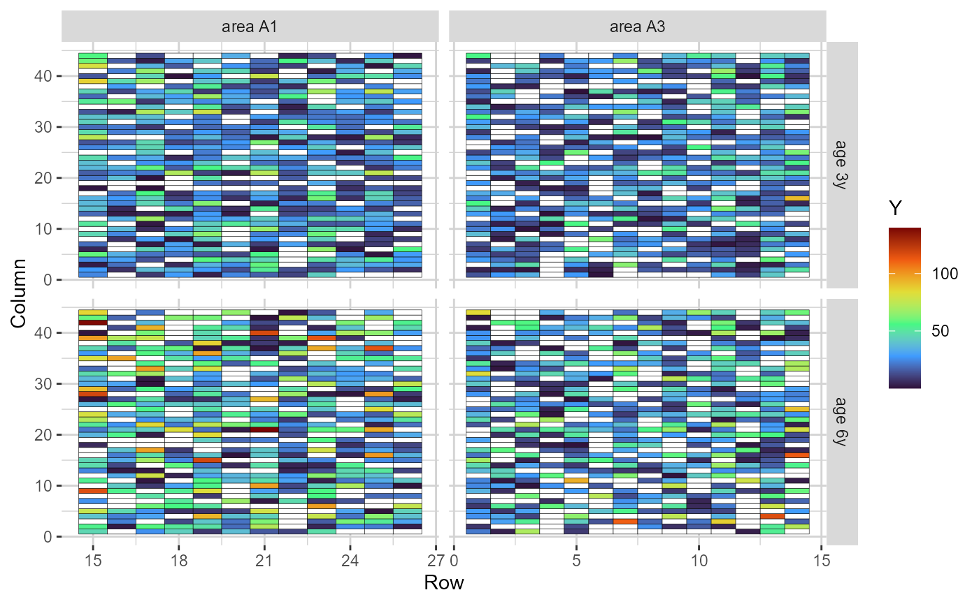

Heatmap representing the grid, in which the cells are filled according to the phenotype value of each plot (blank cells are missing values)

plot(comp_mat, category = "boxplot") + theme(axis.text.x = element_blank())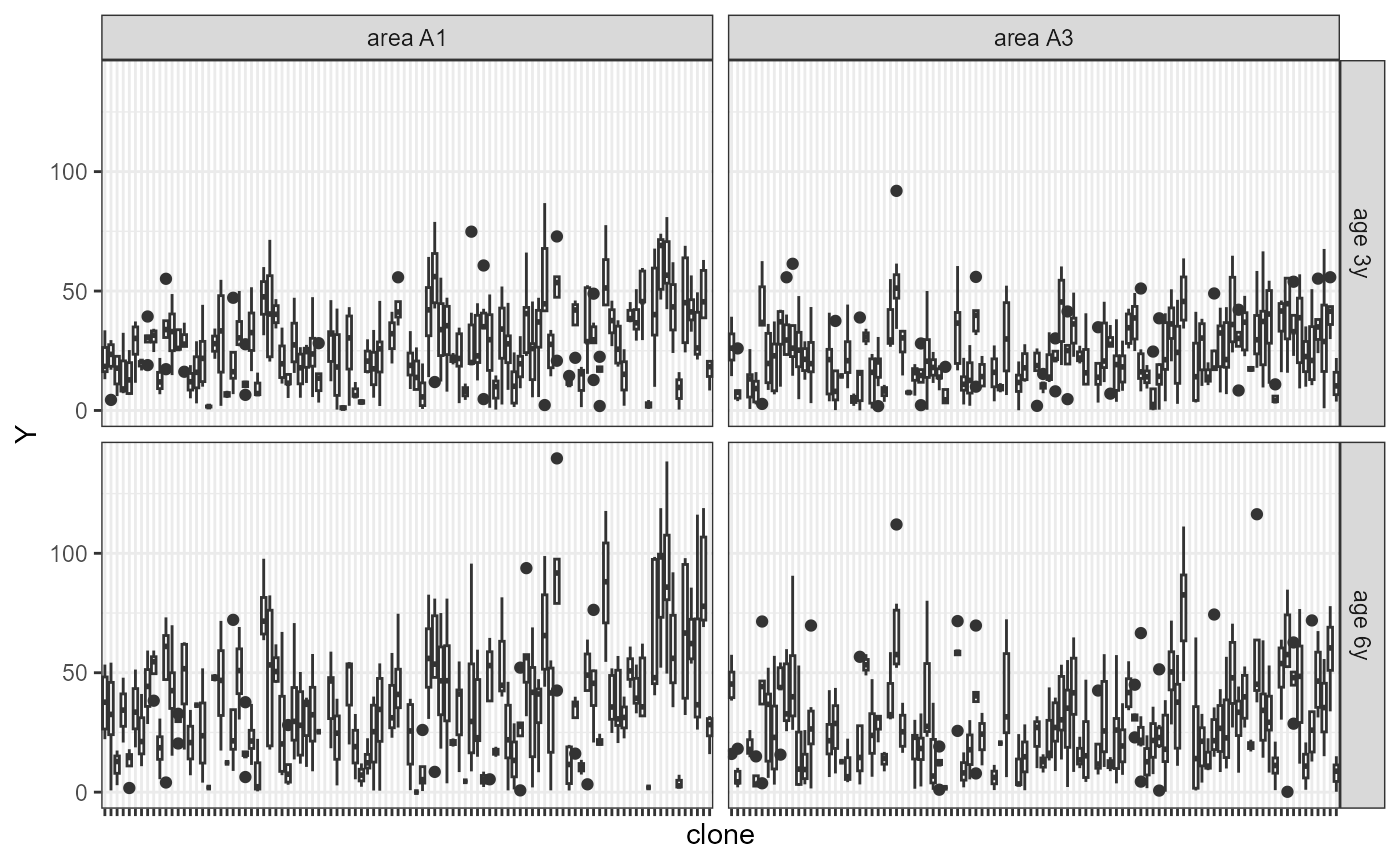

Boxplots depicting the phenotypic performance (y-axis) of each selection candidate (x-axis). The candidates’ names were removed for better visualization

The summary(comprepfor) function returns the number of phenotypic records, number of selection candidates, number of rows and columns, and the number of ages and areas.

summary(comp_mat)
#>    MAI clone row col age area
#> 1 2288   100  26  44   2    2

Fitting the model

A general multi-age spatial-genetic competition model can be represented by:

$\mathbf{y} = \mathbf{X} \boldsymbol{\beta} + \mathbf{Z}_g \mathbf{g} + \mathbf{Z}_c \mathbf{c} + \mathbf{Z}_p \mathbf{p} + \boldsymbol{\varepsilon}$

where $\mathbf{y}$ is the vector of phenotypic records, $\boldsymbol{\beta}$ is the vector of fixed effects, $\mathbf{g}$ is the vector of direct genetic effects (DGE) nested within ages, $\mathbf{c}$ is the vector of indirect genetic effects (IGE) nested within ages, $\mathbf{p}$ is the vector of other random effects, and $\boldsymbol{\varepsilon}$ is the vector of spatially correlated errors. $\mathbf{X}$ is the incidence matrix of the fixed effects, $\mathbf{Z}_g$ is the DGE incidence matrix, $\mathbf{Z}_c$ is the IGE incidence matrix (built using prepfor), and $\mathbf{Z}_p$ is the design matrix of other random effects. The dimensions of $\mathbf{Z}_c$ are the same as $\mathbf{Z}_g$ . The variance-covariance structure of both $\mathbf{g}$ and $\mathbf{c}$ is the compound symmetry, meaning that the equation above estimates their main effects and their interaction with the different ages. The within-age DGE and IGE can be accessed by adding the main effect to its corresponding interaction effect from a specific age. The heterogeneous (per-age) spatially correlated errors are distributed as $\boldsymbol{\varepsilon} \sim \mathcal{N}\{\mathbf{0}, \oplus_{m=1}^M{\sigma^2_{\varepsilon_m} \left( \boldsymbol{AR1}_{C_m} \otimes \boldsymbol{AR1}_{R_m} \right)}\}$ , where $\sigma^2_\varepsilon$ is the spatially correlated residual variance, $\mathbf{AR1}(\rho_C)$ and $\mathbf{AR1}(\rho_R)$ are the first-order autoregressive correlation matrices in the column and row directions, $\otimes$ is the Kronecker product, and $\oplus$ is the direct sum. If area is not NULL (like in the example), heterogeneous residual variances and particular autocorrelations are also obtained per area. If cor = TRUE (default, see below), the function will fit a model in which $\mathbf{g}$ and $\mathbf{c}$ are correlated outcomes of the genotypic effects decomposition.

The function that fits the genetic-competition linear mixed model uses the average information algorithm implemented in the asreml package (The VSNi Team 2023). Check the function’s structure using the example dataset:

model = asr_ma(
  prep.out = comp_mat,
  fixed = MAI ~ age,
  random = ~ block:age,
  lrtest = TRUE,
  spatial = TRUE,
  cor = TRUE
)

prep.out is a comprepfor object. fixed is a formula, declared just like is usually done for regular asreml models. random is also a formula, but this argument should just be altered if other random effects than the genotypic effects should be considered in the model. This is because all pre-programmed models already consider DGE and IGE, as previously described. In our example, we added the block effect, which was declared in the effs argument of comprepfor. lrtest defines if hypothesis tests using likelihood ratio tests should be done. spatial determines if a regular genetic competition model (spatial = FALSE) or a spatial-genetic competition model (spatial = TRUE) should be fitted. Finally, cor dictates if the function will fit a model considering the covariance between DGE and IGE (cor = TRUE) or not (cor = FALSE). asr_ma can receive other arguments passed on to the asreml function (see ?asreml for more information). The output of the asr_ma function is an object of classes asreml and compmod. Since it holds the asreml class, it is suitable for using with generic functions like plot, summary, predict, update, resid and others (see help("asreml.object")).

Extracting the results

The function to obtain the main results from the compmod object is called resp, and its structure is exemplified below using the example dataset:

res = resp(
  prep.out = comp_mat,
  model = model,
  weight.tgv = FALSE,
  sd.class = 1
)

model is the compmod object obtained from the asr_ma function. weight.tgv receives a logical value, and determines if the reliability should be used as weight to compute the total genotypic value (TGV) or not. sd.class is a weight to multiply the standard deviation of competition effects when determining the competition classes (defaults to 1). The resp function returns an object (list) of classes comresp and comprepfor. This object is compatible with the generic functions plot, print and summary. A detailed description of the results within the list generated by res is provided below.

Variance components

The data frame with the variance components will yield different results depending on the model. cor(IGE_DGE), which represents the correlation between DGE and IGE; DGE and IGE will always be present in variance component obtained from compmod objects. The residuals will have different forms depending if area is NULL or not in the prepfor function, and if spatial is TRUE or FALSE in the asr_ma function.

res$varcomp

	component	std.error	z.ratio	bound	%ch
block:age	16.2170	5.8367	2.7785	P	0.0
cor(IGE_DGE)	-0.5830	0.1073	-5.4327	U	0.0
DGE	143.2868	23.5141	6.0936	P	0.0
IGE	20.6057	4.5400	4.5387	P	0.0
DGE:age	5.2824	4.4706	1.1816	P	0.2
IGE:age	0.0000	NA	NA	B	NA
R=area_A1:age_3y	177.6881	14.0806	12.6193	P	0.0
R=autocor(row):area_A1:age_3y	0.0784	0.0625	1.2533	U	0.1
R=autocor(col):area_A1:age_3y	-0.1413	0.0637	-2.2199	U	0.0
R=area_A3:age_3y	133.5698	10.2324	13.0536	P	0.0
R=autocor(row):area_A3:age_3y	0.0315	0.0675	0.4666	U	0.8
R=autocor(col):area_A3:age_3y	0.0715	0.0637	1.1225	U	0.1
R=area_A1:age_6y	426.0002	34.0643	12.5058	P	0.0
R=autocor(row):area_A1:age_6y	-0.0313	0.0682	-0.4597	U	0.6
R=autocor(col):area_A1:age_6y	-0.1942	0.0638	-3.0427	U	0.0
R=area_A3:age_6y	244.1681	19.3033	12.6490	P	0.0
R=autocor(row):area_A3:age_6y	-0.0365	0.0751	-0.4866	U	0.7
R=autocor(col):area_A3:age_6y	0.0759	0.0693	1.0943	U	0.2

Likelihood ratio tests

Available only if lrt = TRUE in the asr_ma function.

res$lrt

effect	LR-statistic	Pr(Chisq)
DGE	109.8212115	0.0000000
IGE	56.7154599	0.0000000
DGE:age	2.0228651	0.0774733
IGE:age	-0.0000951	0.5000000

Heritabilities

Available if cor = TRUE in the function asr. Contain the DGE heritability and total heritability Bijma, Muir, and Van Arendonk (2007). The first is the portion of the total variance that refers to the DGE. The latter is a ratio between the sum of the total heritable components against the phenotypic variance, and it is an adjusted estimate of the heritability that considers the competition effects and the covariance between DGE and IGE. The expressions for these heritabilities are given below:

$H^2_g = \frac{\hat{\sigma}^2_g}{\hat{\sigma}^2_y}$ $H^2_t = \frac{\hat{\sigma}^2_g + 2\times \hat{\phi} \times \hat{\sigma}_{gc} + \hat{\phi}^2 \times \hat{\sigma}^2_c}{\hat{\sigma}^2_y}$ with $\sigma^2_y$ being the total phenotypic variance.

res$heritability

	H2direct	H2total
area_A1:age_3y	0.395	0.296
area_A3:age_3y	0.449	0.337
area_A1:age_6y	0.234	0.176
area_A3:age_6y	0.334	0.250

Since area is not NULL in our example, and the model estimates heterogeneous residual variances, the heritabilities are particularized per area.

BLUPs

When genetic competition effects are statistically significant, the most appropriate selection unit is the TGV, given by:

${TGV}_v = \hat{g}_v + \hat{\phi} \times \hat{c}_v$ where $\hat{g}_v$ and $\hat{c}_v$ are the DGE and IGE of the $v^{th}$ candidate, respectively. If weight.tgv = TRUE in the resp function, the weighted TGV is computed as follows:

${wTGV}_v = \hat{g}_v \times r_{g_v}^2 + \hat{\phi} \times \hat{c}_v \times r_{c_v}^2$ with $r_{g_v}^2$ and $r_{c_v}^2$ being the reliabilities of DGE and IGE, respectively.

The comresp object has a data frame containing the DGE and IGE, their standard errors, the competition class of each genotype and the TGV. In the multi-age case, there are two lists: one containing the main effects, and other with the within-ages effects (main + interaction). If other random effects were declared in the model, there will be a further data frame with their BLUPs.

head(res$blups$main)

clone	DGE	se.DGE	rel.DGE	IGE	se.IGE	rel.IGE	class	TGV
C099	24.616	3.578	0.911	-0.799	2.461	0.706	Homeostatic	22.752
C087	13.201	4.120	0.882	2.194	2.477	0.702	Homeostatic	18.316
C083	22.710	3.620	0.909	-3.442	2.510	0.694	Homeostatic	14.685
C028	26.150	3.475	0.916	-6.024	2.636	0.663	Aggressive	12.104
C066	8.528	3.635	0.908	1.335	2.334	0.736	Homeostatic	11.641
C092	28.117	3.666	0.906	-7.119	2.646	0.660	Aggressive	11.520

head(res$blups$within)

clone	age	DGE	se.DGE	rel.DGE	IGE	se.IGE	rel.IGE	class	TGV
C099	6y	27.029	2.172	0.967	-0.799	0.001	1	Homeostatic	25.198
C099	3y	23.506	2.159	0.967	-0.799	0.001	1	Aggressive	21.611
C087	6y	14.494	2.208	0.966	2.194	0.001	1	Homeostatic	19.521
C087	3y	12.833	2.194	0.966	2.194	0.001	1	Homeostatic	18.035
C083	6y	23.676	2.176	0.967	-3.442	0.001	1	Homeostatic	15.789
C083	3y	22.714	2.163	0.967	-3.442	0.001	1	Homeostatic	14.552

From this data frame, several information can be extracted. In the generic function plot, use the argument level to control if the plot should illustrate information from main effects (level = "main") or within-ages effects (level = "within"). If level = "within", another argument, age, will further define if all ages should be plotted together (age = "all") or separately (age = name of a specific age). Check out below.

Competition classes

The higher the IGE, the more aggressive is the genotype. Here, we use a modified version of the classification proposed by Filipe M. Ferreira et al. (2023) to define competition classes:

$\text{Classes} = \begin{cases} \bar{c} - (\tau) sd(c) < \hat{c}_v < \bar{c} + (\tau) sd(c) \rightarrow \text{Homoeostatic} \\ \hat{c}_v > \bar{c} + (\tau) sd(c) \rightarrow \text{Sensitive} \\ \hat{c}_v < \bar{c} - (\tau) sd(c) \rightarrow \text{Aggresive} \end{cases}$ with $\bar{c}$ being the mean IGE in the population, $\hat{c}_v$ the IGE of the $v^{th}$ genotype, $sd(c)$ the IGE’s standard deviation, and $\tau$ a weight defining the thresholds to declare if a genotype is aggressive, homoeostatic or sensitive.

This classification is illustrated using a density plot, a scatter plot and a heat map representing the field grid. These plots aid in the investigation of the relationship between DGE and IGE, how this dynamics are related to classification, and how aggressive, homoeostatic and sensitive are distributed in the field.

plot(res, category = "class", level = "main")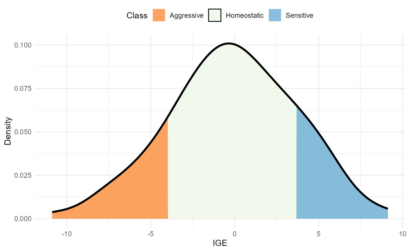

Density of IGE values. The area within the distribution is filled according to the competition class

plot(res, category = "DGEvIGE", level = "within")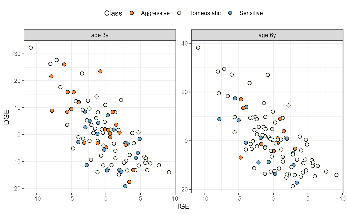

Relationship between IGE (x-axis) and DGE (y-axis). The dots are coloured according to the competition class.

plot(res, category = "grid.class", level = "within", age = "6y")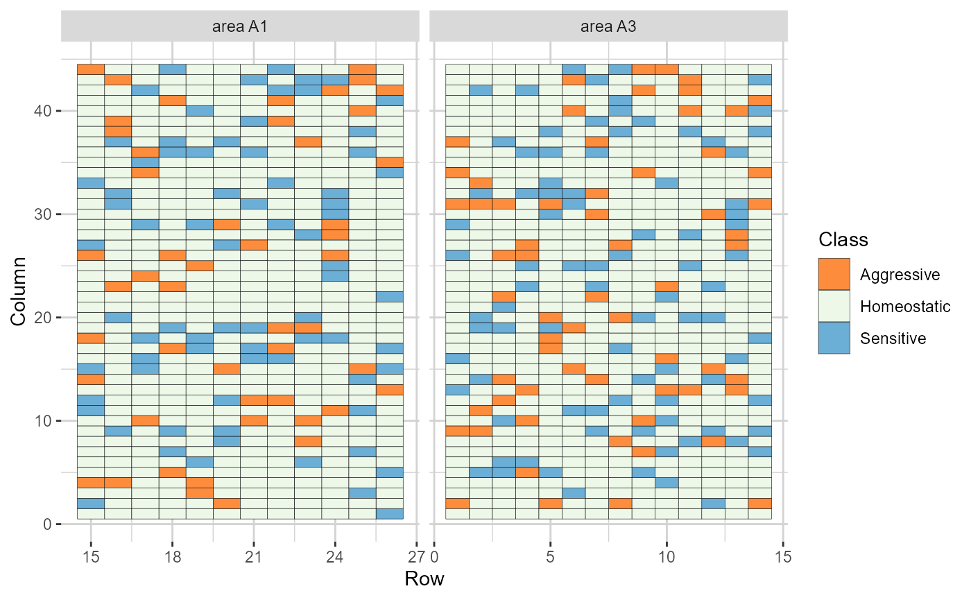

Heatmap representations of the field trial, with cells filled according to the competition class of each genotype

Ranking

Three possible rankings are possible: based on the DGE, the IGE, or the TGV. Note that DGE and IGE have different reliabilities, with DGE’s being usually higher. It is advisable to take this into consideration when making decisions.

plot(res, category = "DGE.IGE", level = "main") + 
  theme(axis.text.x = element_text(size = 4, vjust = .5, hjust = 1))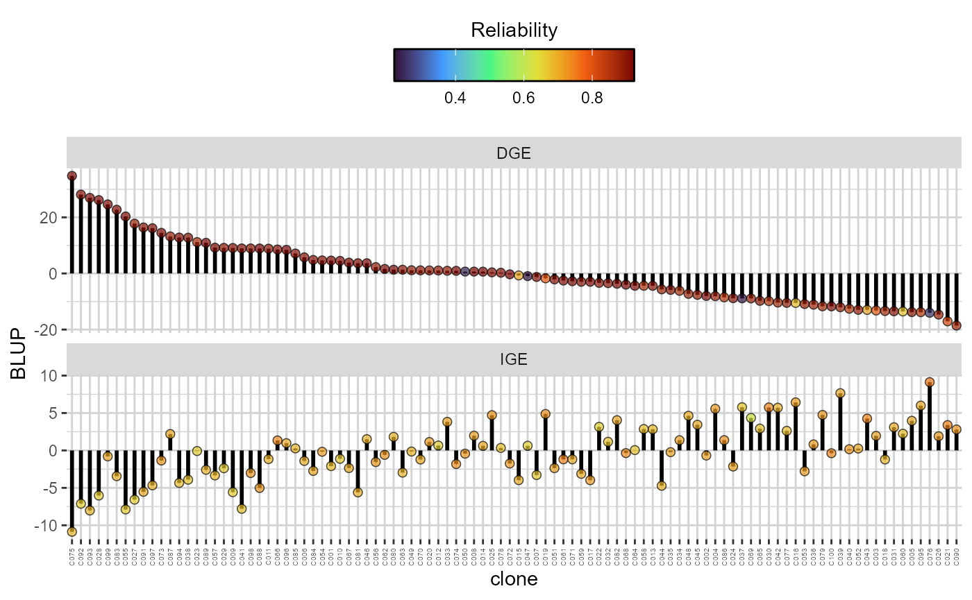

Direct (DGE) and indirect (IGE) genotypic effects ( extit{y}-axis) of each candidate. The plots are in descending order according to the DGE. The colour of the dots reflects the reliability of both the DGE and IGE for each genotype

plot(res, category = "TGV", level = "within", age = "3y") + 
  theme(axis.text.x = element_text(size = 4, vjust = .5, hjust = 1))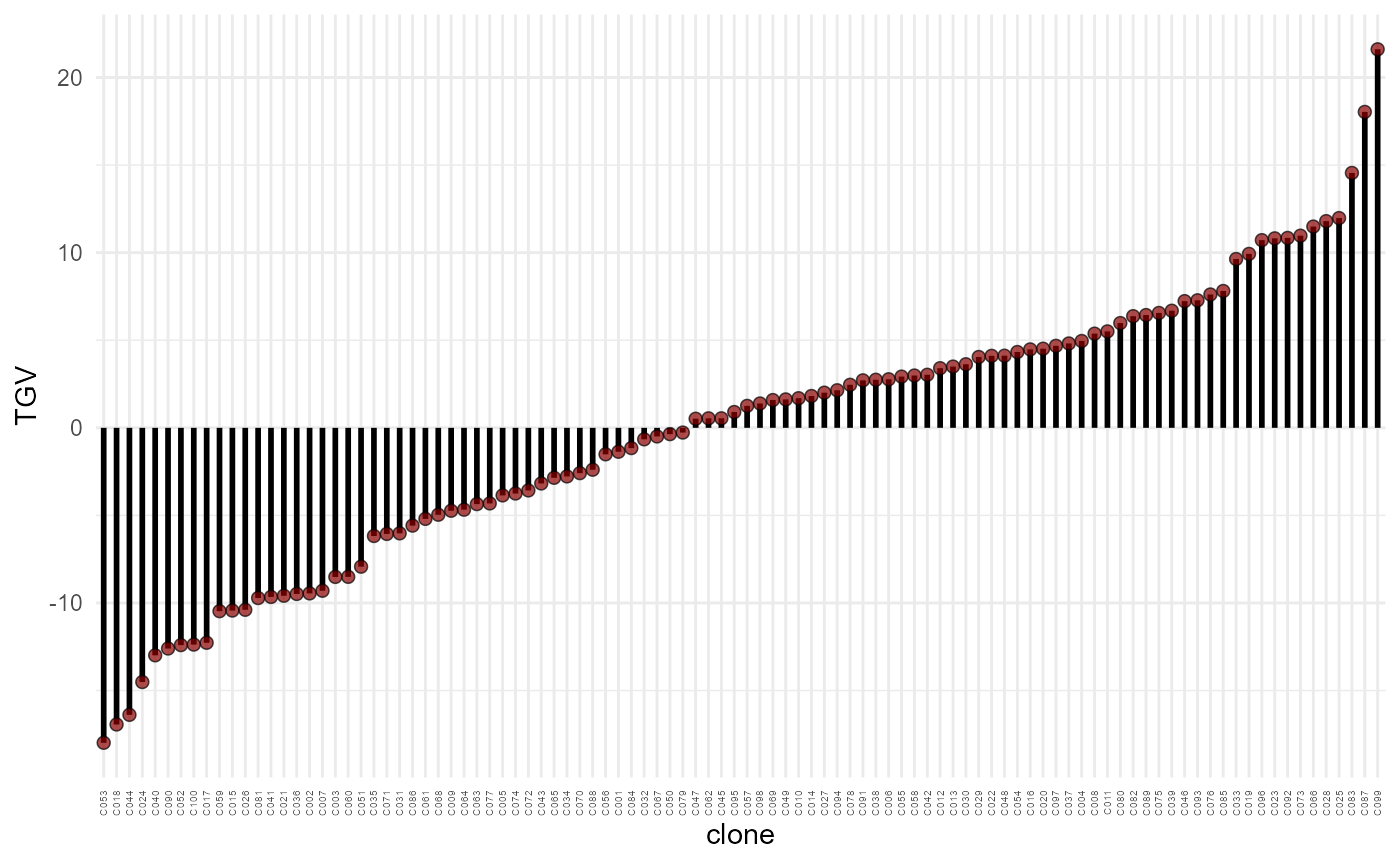

Total genotypic value (TGV) (y-axis) of each candidate (x-axis), in increasing order

The distribution of high-performance and/or competitive candidates is also illustrated.

plot(res, category = "grid.dge", level = "within", age = "all")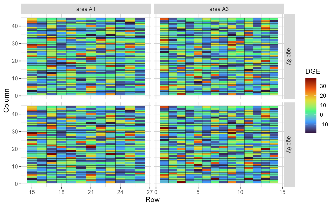

Heatmap representations of the field trial, with cells filled according to the direct genotypic effect (DGE) of each genotype

plot(res, category = "grid.ige", level = "within", age = "3y")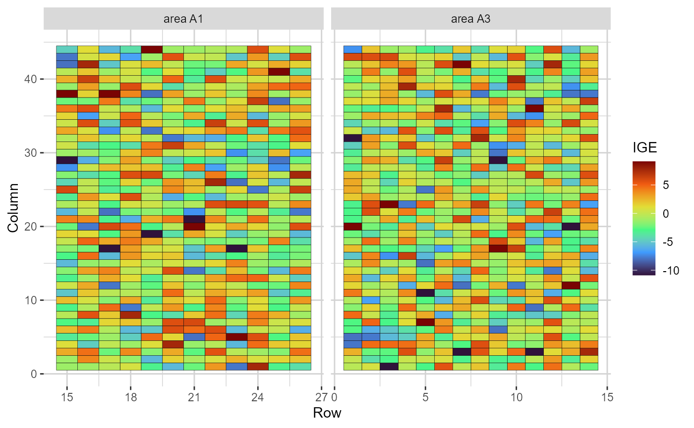

Heatmap representations of the field trial, with cells filled according to the indirect genotypic effect (IGE) of each genotype

Number of different neighbours

The number of different genotypes as neighbours of the candidates can be evaluated by the figure below. In the example dataset, almost all clones neighboured each other, and most of them had homoeostatic neighbours.

plot(res, category = "nneigh", level = "within", age = "all")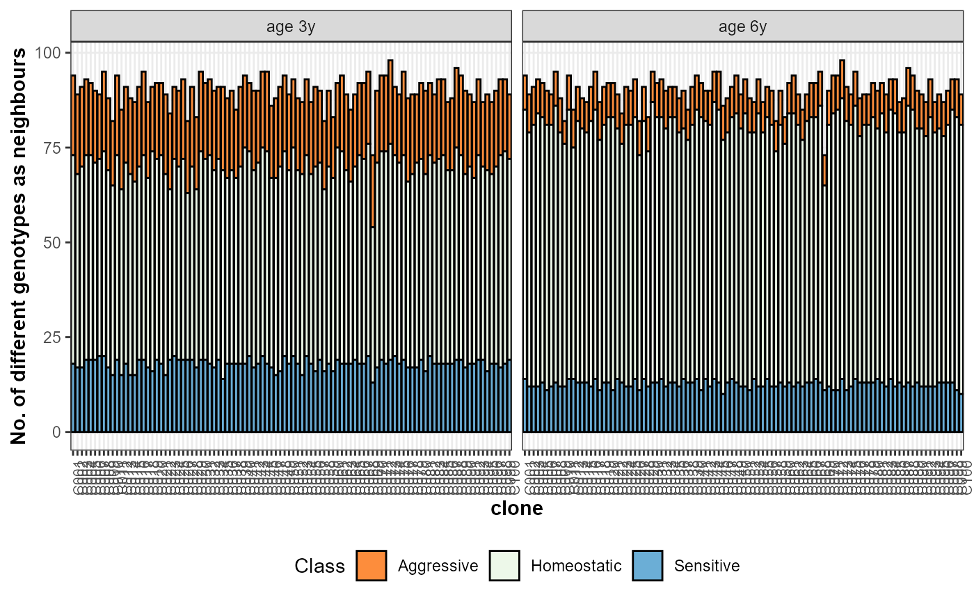

Number of different genotypes as neighbors (total and per competition class) of each selection candidate

Error distribution

The last plot available for objects of class compresp is a heatmap coloured according to the residual value of each plot. This is useful to observe possible trends in the field.

plot(res, category = "grid.res", level = "main")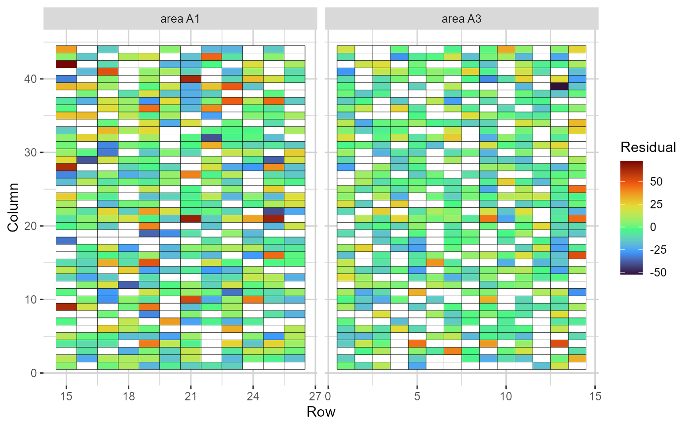

Heatmap representations of the field trial, with cells filled according to the residual value of each plot. Blank cells are missing values

References

Bijma, Piter, William M. Muir, and Johan A. M. Van Arendonk. 2007. “Multilevel Selection 1: Quantitative Genetics of Inheritance and Response to Selection.” Genetics 175 (1): 277–88. https://doi.org/10.1534/genetics.106.062711.

Cappa, Eduardo P., and R. J. C. Cantet. 2008. “Direct and Competition Additive Effects in Tree Breeding: Bayesian Estimation from an Individual Tree Mixed Model.” Silvae Genetica 57 (2): 45–56. https://doi.org/10.1515/sg-2008-0008.

Chaves, Saulo F. S., Filipe M. Ferreira, Getulio C. Ferreira, Salvador A. Gezan, and Kaio Olimpio G. Dias. 2025. “Incorporating Spatial and Genetic Competition into Breeding Pipelines with the R Package Gencomp.” Heredity, January, 1–13. https://doi.org/10.1038/s41437-024-00743-9.

Costa e Silva, João Costa, and Richard J. Kerr. 2013. “Accounting for Competition in Genetic Analysis, with Particular Emphasis on Forest Genetic Trials.” Tree Genetics & Genomes 9 (1): 1–17. https://doi.org/10.1007/s11295-012-0521-8.

Ferreira, Filipe Manoel, Saulo Fabrício Silva Chaves, Osmarino Pires Santos, Andrei Caíque Pires Nunes, Evandro Vagner Tambarussi, Guilherme Silva Pereira, Gleison Augusto Santos, Leonardo Lopes Bhering, and Kaio Olimpio Graças Dias. 2024. “Competition Effects Can Mislead Selection in Eucalypt Breeding Trials.” Forest Ecology and Management 561: 121892. https://doi.org/10.1016/j.foreco.2024.121892.

Ferreira, Filipe M., Saulo F. S. Chaves, Leonardo L. Bhering, Rodrigo S. Alves, Elizabete K. Takahashi, João E. Sousa, Marcos D. V. Resende, et al. 2023. “A Novel Strategy to Predict Clonal Composites by Jointly Modeling Spatial Variation and Genetic Competition.” Forest Ecology and Management 548: 121393. https://doi.org/10.1016/j.foreco.2023.121393.

Muir, William M. 2005. “Incorporation of Competitive Effects in Forest Tree or Animal Breeding Programs.” Genetics 170 (3): 1247–59. https://doi.org/10.1534/genetics.104.035956.

The VSNi Team. 2023. Asreml: Fits Linear Mixed Models Using REML. www.vsni.co.uk.

Wickham, Hadley. 2016. Ggplot2: Elegant Graphics for Data Analysis. Springer-Verlag New York. https://ggplot2.tidyverse.org.

Saulo F. S. Chaves

2025-01-21